Chapter 4 Digression: Linear Regression and how to apply it

library("stargazer")

In the social sciences (in fact, in all sciences) linear regressions (also called OLS or ordinary least squares) or one of its relatives is the most used empirical research tool there is. Why? It is relatively simple, computationally fast, easy to interpret and relies on a relatively weak set of assumptions. Unfortunately, the assumptions needed to be able to apply linear regression, are often not well understood: both in the social sciences and beyond. Moreover, students in the social sciences typically get little guidance in how to apply linear regression in practice and how to interpret the results. Note that this does not have anything to do with the specific software students use, but more with that fact that regression techniques in a wide number of situations (courses) are just not given (apart from statistical or research methods courses). However, given the fact that data becomes increasingly more available, knowing when to use regression techniques, how to apply them and especially how to interpret and assess them is now becoming an issue of paramount importance. Or, perhaps more compelling, you need them to write your thesis.

In this chapter, I will first focus in section 4.1 on the essential theory behind regression analysis. I really keep it to the bare minimum. But if you understand these basics, I would argue that you understand more than 75% of the theorical background (the rest if just nitty-gritty). Section 4.2 will focus on applications of linear regression, specification issues (how many variables) and how to interpret the results.

4.1 Theoretical background

This subsection first deals with the model (what are you trying to explain), then about the three critical assumptions of (ordinary) least squares, discusses subsequently typical situations when these assumptions are violated, and finishes with a discussion about less important stuff (on which, alas, quite some attention is given in bachelor courses).

Before we start, I would like to make one important remark. In general, statistical models can be used for (i) finding statistical relations, finding (ii) causal relations and for (iii) predicting. All three uses require the same assumptions, but have different focuses. In statistics, generally the focus is on finding statistical relations, such as whether the Dutch population is on average taller then the German population. In economics the focus is very much on finding causal relations, so the need for explanatory power is not very large. Models that do not explain much (where the \(R^2\)’s are low, say \(<\) 0.2) are just as good as models that explain quite a lot, as long as the least squares assumptions hold. In transportation science in general (and other disciplines that deals with making large models) predictions and thus explanatory power is key. Here it is now very important that you perfectly understand what causes what as long as out-of-sample predicting is good (say for predicting future commuting flows).

I usually have finding causal relations in mind when talking about least squares (already difficult enough), but note again that the same least squares assumptions, in some form or another, should hold when you want to predict or want to find statistical relations.

4.1.1 The model

Assume we are interested in the effect of the weight of a car on the fuel efficiency of the car (measured in miles per gallon). We state the following univariate regression model: \[ y_i = \alpha + \beta x_i + \epsilon_i, \] where \(y\) denotes the fuel efficiency of the car, \(x\) denotes the weight of the car and subscript \(i\) stands for the \(i\)-th observation. \(\alpha\) and \(\beta\) are the parameters of the model and they are unknown so they have to be estimated. \(\epsilon\) is a so-called error term and denotes all the variation that is not captured by our two variables (\(\alpha\) and \(\beta\)) and our weight of the car variable \(x\).

The following observations are very important:

What is on the left hand side of the \(=\) sign is what is to be explained (in this case miles per gallon). What is on the right hand side is what we use to explain \(y\); in this case being \(x\), the weight of the car.
The parameters \(\alpha\) en \(\beta\) constitute a linear relation between \(x\) and \(y\)
The parameter \(\alpha\) is the constant and in the univariate setting denotes where the linear relation crosses the \(y\)-axis.
\(\beta\) gives the impact of \(x\) on \(y\). Because it is a linear relation, the effect is simple. One unit change of \(x\) is associated with a \(\beta\) change of \(y\). In general, we can say that \(\beta\) is equal to the marginal effect (\(\frac{\partial y}{\partial x}\)). Moreover, in a univariate setting \(\beta\) denotes the slope of the relation between \(x\) and \(y\).
The regression error term \(\epsilon\) gives all variation that is not captured by our model, so \(y_i -(\alpha + \beta x_i) = \epsilon_i\). In this case, weight of the car most likely does not capture all variation in miles per gallon, so quite some variation is left in \(\epsilon\). Something else is captured as well by \(\epsilon\) and that is the measurement error of \(y\). So, if we have not measured miles per gallon precisely enough then that variation is captured as well by \(\epsilon\).

Now, let’s assume that we want to incorporate another variable (say the number of cylinders, denoted by \(c\)), because we think that that variable is very important as well in explaining miles per gallon. Then we get the following multivariate regression model: \[ y_i = \alpha + \beta_1 x_i + \beta_2 c_i + \epsilon_i, \] where we now have two variables on the right hand side (\(x_i\) and \(c_i\)) and three parameters (\(\alpha\), \(\beta_1\) and \(\beta_2\)). In effect nothing changes with the intuition behind the model. Except for the interpretation of the parameter \(\beta_1\) (and thus also \(\beta_2\)). Parameter \(\beta_1\) now measures the impact of \(x\) on \(y\) holding \(c\) constant. So, multivariate regression models is nothing more (and less) than controlling for other factors. And we see later why that is very important.

4.1.2 The least squares assumptions

We are interested in the effect of the weight of the car on fuel efficiency and,therefore, our estimate of \(\beta_1\) should be very close to the true \(\beta_1\), especially when we have a large number of observations. Regression is great and utterly brilliant in finding this estimate, as long as the following three least squares assumptions hold:

There are no large outliers.
All left hand side (in this case \(y\)) and right side variables (in this case \(x\) and \(c\)) are i.i.d.
For the error term the following must hold: \(E[\epsilon|X=x] = 0\).

The first one is easy to understand. OLS is very sensitive to large outliers in the dataset. It is therefore always good to look for outliers and think whether they are real observations or perhaps typo’s (in Excel or something). Do not throw outliers immediately away but check whether they are correct.

The second is relatively easy to understand as well (but not that easy to uphold in practice). i.i.d. in this case stands for independently and identically distributed. This basically means that the observations in your dataset are independent from each other: in other words, the observations should have been correctly sampled.

The third looks the most horrible, and, to be quite honest, is so–both in theory as in reality. This is also the assumption that is least well understood; below, I will give some intuition what this assumptions stands for. And especially in assessing whether regression output is correct (is your estimate really close to \(\beta_1\)) this assumption is crucial.

4.1.3 Possible violations and how to spot them

A violation of the first assumption is usually easy to spot. There is a very strange outlier somewhere. But this also signifies the importance of analysing descriptive statistics, including means, maximums and minimums, scatterplots and histograms.

Whether your data is not i.i.d. can come because of a couple of reasons. The most straightforward is getting your data via snowballing (asking your friends and families using facebook to fill in a questionnaire and to ask their friends and families to do so as well). Usually, this means that you have a very specific sample and that the estimate you get is not close to the true value for the whole population. Observations might also be dependent upon each other, because of unobserved factors. In our case, it might be that a type of cars (American) are less fuel efficient than other cars (European).

Another typical violation of the i.i.d. assumption is in time-series, where what happened in the previous period might have a large effect on the current period.

In general, however, violations of the i.i.d. property are not that devastating for your model as long as you are only interested in finding the true \(\beta_1\): namely, it usually only affects the precision of your estimate (the standard error) and not the estimate itself. When this assumption is violated, we therefore say that the estimate is inefficient. When you want to predict, however, this assumption is crucial, as you would like your estimate to be as precise as possible.

When the third assumption is violated, we say that our estimate is biased, in other words wrong: our parameter estimate does not come close to the true parameter. And this happens more often than not. So, what does \(E[\epsilon|X=x] = 0\) actually mean. Loosely speaking, the parameters on the right hand side (in our case \(x\) and \(c\)) on the one hand and the error term (\(\epsilon\)) on the other hand are not allowed to be correlated. There are several ways how this might happen, from which the following are in our case the most relevant:

Reverse causality: \(x\) impacts \(y\), but \(y\) might impact \(x\) as well. This is the classical chicken and egg problem. Do firms perform better because of good management, or do good managers go to the better performing firms?
Unobserved heterogeneity bias: there are factors that are not in the model but influence both \(x\) and \(y\). For example, if american cars have both an influence on fuel efficiency and weight of the cars then the estimate that we find is not close to the true value of \(\beta_1\).
Misspecification: we assume that our model is linear, but it actually is not. Then, again, our estimate that we find is not close to the true value of \(\beta_1\).

There are other sources of violations, but in this case, these are the most important ones. Reverse causality is usually hard to correct for, but unobserved heterogeneity bias is luckily easier. Namely, we add relevant control variables (as we did with \(c\)). In this case we can minimize possible unobserved heterogeity bias. Misspefications are in general as well relatively easy to correct for. From our descriptive statistics and scatterplot we usually can infer the relation between \(x\) and \(y\) and control for possible nonlinearities by using (natural) logarithms and squared terms.

As a sidenote, natural logarithms are the ones most used for various reasons not discussed here. If we take the logarithm of both sides then for our univariate regression we get: \[ \ln(y_i) = \alpha + \beta \ln(x_i) + \epsilon_i, \] and all the aforementioned rules and assumptions still apply. But there is something peculiar to this regression. Namely, if we are interested in the marginal effect (\(\frac{\partial y}{\partial x}\)), we get the following: \[ \frac{\partial y}{\partial x} = \frac{\partial e^{\ln(y_t)}}{\partial x} = \frac{\partial e^{(\alpha + \beta \ln(x_i) + \epsilon_i)}}{\partial x} = \frac{\beta}{x}e^{(\alpha + \beta \ln(x_i) + \epsilon_i)} = \frac{\beta}{x}y, \] In other words: \[ \beta = \frac{\partial y}{\partial x} \frac{x}{y} \] which is simply the elasticity between \(x\) and \(y\). So, if there are logarithms on both the left and right hand side then the parameters (the \(\beta\)’s) denotes elasticities.

4.1.4 Normality, heteroskedasticity and multicollinearity

Until now, we have not discussed the concepts normality, heteroskedasticity and multicollinearity. That is simply because they are not that relevant (as long as we have enough observations, typically above 40). The validity of OLS hinges just upon the three assumptions mentioned above (and they are already difficult enough). In fact, if the three assumptions are satisfied, then, as an outcome, the parameters (\(\beta\)) are normally distributed. It goes to far to explain why (the theorems required for this are deeply fundamental to statistics), but in any case, normality is not a core OLS assumption. It would be nice if both \(y\) and \(x\) are normally distributed because then the standard errors are minimized, but again, whether the estimate of \(\beta\) you find is correct or not (biased or unbiased) does not depend on normality assumptions.

Heteroskedasticy (in other words your standard errors are not constant) as well leads to quite some confusion. In general heteroskedasticity only leads to inefficient estimates (so only affects the standard errors). Nothing more, nothing less. And there are corrections for that (robust standard errors in Stata and similar procedures in R), so that nobody needs to care anymore about heteroskedasticity.

Finally, there is multicollinearity. And this comes in two flavours: perfect and imperfect multicollinearity. Perfect multicollinearity occurs, e.g., when your model contains two identical variables. Then, OLS can not decide which one to use and usually one of the variables is dropped, or your computer program gives an error (computer says no).

Imperfect multicollinearity occurs when two variables are highly (but not perfectly) correlated. This occurs less often than one may think. Variables that are highly correlated (say \(age\) and \(age^2\)) can be perfectly incorporated in a model. Only when the correlation becomes very high (say above 95% or even higher) then something strange happens: the standard errors get very large. Why? That is because of the definition mentioned above. Parameter \(\beta_1\) measures the impact of \(x\) on \(y\) holding \(c\) constant. But if \(x\) and \(c\) are very highly correlated and you control for \(c\), then not much variation is left over for \(x\). So, \(c\) actually removes the variation within the variable \(x\). This always happens, and there is a trade-off between adding more variables and leaving enough variation (note that there is always correlation between variables), but usually it all goes fine. Good judgement and sound thinking typically helps more than strange statistics (say VIF?).

4.2 Applications of linear regression

This section gives an application of regression analysis. Assume we are still interested in the effect of the weight of a car on the fuel efficiency of the car (measures in miles per gallon). We have found a dataset (internal in R), so the first thing we have to do is look at the descriptives of the dataset.

4.2.1 Descriptives

The build-in dataset mtcars has, besides several other variables, information on weight of a car (in 1000 lbs or in about 450 kilos) and miles per gallon. With the following command head() we can look at the first 6 observations.

head(mtcars)

##                    mpg cyl disp  hp drat    wt  qsec vs am gear carb
## Mazda RX4         21.0   6  160 110 3.90 2.620 16.46  0  1    4    4
## Mazda RX4 Wag     21.0   6  160 110 3.90 2.875 17.02  0  1    4    4
## Datsun 710        22.8   4  108  93 3.85 2.320 18.61  1  1    4    1
## Hornet 4 Drive    21.4   6  258 110 3.08 3.215 19.44  1  0    3    1
## Hornet Sportabout 18.7   8  360 175 3.15 3.440 17.02  0  0    3    2
## Valiant           18.1   6  225 105 2.76 3.460 20.22  1  0    3    1

Again, we are interested in the relation weight of a car (the variable wt) and miles per gallon (the variable mpg). Note, that in his case mpg is the first column and wt is the sixth column. (The column with car names above is not a real variable, but are the row names). Recall that the command c() combines stuff, so we can look at the summary statistics of the variables we are only interested in by:

summary(mtcars[,c(1,6)])

##       mpg              wt       
##  Min.   :10.40   Min.   :1.513  
##  1st Qu.:15.43   1st Qu.:2.581  
##  Median :19.20   Median :3.325  
##  Mean   :20.09   Mean   :3.217  
##  3rd Qu.:22.80   3rd Qu.:3.610  
##  Max.   :33.90   Max.   :5.424

There does not seem to be anything out of the ordinary here, but to be sure, we construct a scatterplot between weight of the car and miles per gallon.

plot(mpg~wt, mtcars)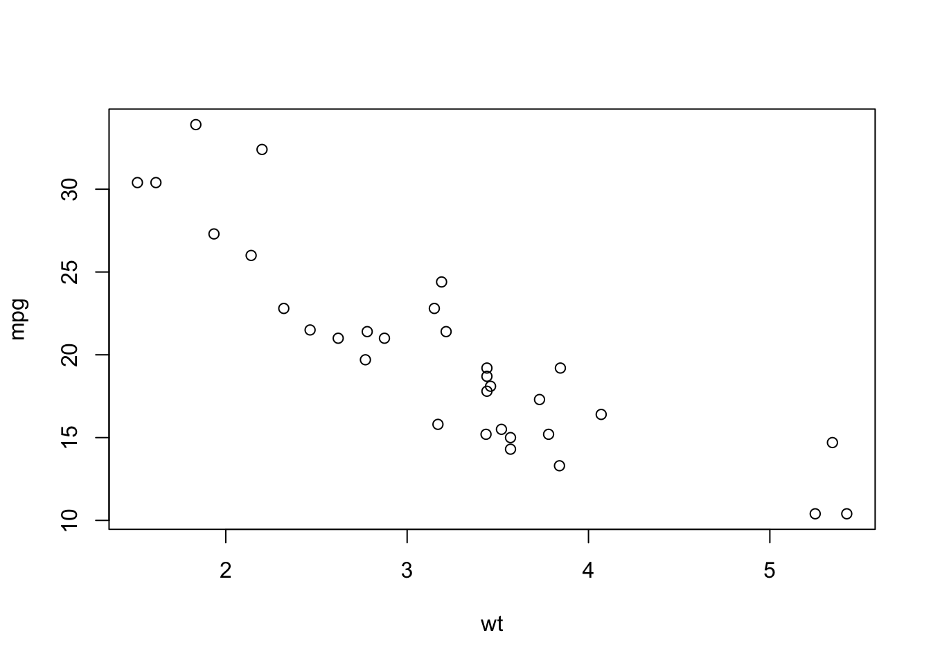

Figure 4.1: A scatterplog between miles per gallon and car weight.

So, there do not seem to be many outliers here. Moreover, as we would expect, there seems to be a downward sloping relation between weight of the car and miles per gallon (hopefully you agree, that this makes sense). To quantify this relation, the next subsection will perform a least squares estimation.

4.2.2 Baseline model

So, if we are only interested in the relation between weight of a car (the variable wt) and miles per gallon, we can easily perform the following regression (recall again that the command lm() performs a least squares estimation and that <- denotes an assignment to a variable:

baselinemodel <- lm(mpg~wt, mtcars)
summary(baselinemodel)

## 
## Call:
## lm(formula = mpg ~ wt, data = mtcars)
## 
## Residuals:
##     Min      1Q  Median      3Q     Max 
## -4.5432 -2.3647 -0.1252  1.4096  6.8727 
## 
## Coefficients:
##             Estimate Std. Error t value Pr(>|t|)    
## (Intercept)  37.2851     1.8776  19.858  < 2e-16 ***
## wt           -5.3445     0.5591  -9.559 1.29e-10 ***
## ---
## Signif. codes:  0 '***' 0.001 '**' 0.01 '*' 0.05 '.' 0.1 ' ' 1
## 
## Residual standard error: 3.046 on 30 degrees of freedom
## Multiple R-squared:  0.7528, Adjusted R-squared:  0.7446 
## F-statistic: 91.38 on 1 and 30 DF,  p-value: 1.294e-10

At this point it is good to stop and see what we have got. We have the formula call (we know this one), some stuff about the residuals, stuff about the coefficients (most important for us), and some diagnostics (including the notorious \(R^2\)). We zoom in on the results about the coefficients. We have an estimation of the intercept (our \(\alpha\) of above) and of wt (our \(\beta\) of above). For both, we have as well a standard error, a \(t\)-value, a probability and a bunch of stars. What do they all mean again? We focus on wt here (typically we are less interested in the constant or intercept).

The estimate is easy; that is \(\beta\) or the marginal effect of \(x\) on \(y\). So, increasing \(x\) with 1 (or with a 1000 lbs) decreases the miles per gallon with 5.3445 (which is quite a lot).

The standard error denotes the precision of the estimate. As a rule of thumb: you know with 95% centainty that the true value of \(\beta\) lies within the interval [estimate \(- 2 \times\) standard error, estimate \(+ 2 \times\) standard error]. The standard error is very important and is used to test possible values of the parameter. One of the most important tests is whether \(\beta=0\). Why? Because, if \(\beta=0\) then the variable wt does nothing on mpg. This specific test is always denoted by the \(t\)-value, its associated probability and the corresponding star thingies. In this case, the \(t\)-value is high in an absolute sense, so it is very improbable that the estimate could be zero (somehting like a probability of 0.0000000001 which is small indeed), and the stars neatly indicate that this probability (of \(\beta=0\)) is smaller than 0.001.

One nice trick is to plot the regression line in the scatterplot above. One can do so by the command abline() or:

plot(mpg~wt, mtcars)
abline(lm(mpg~wt, mtcars))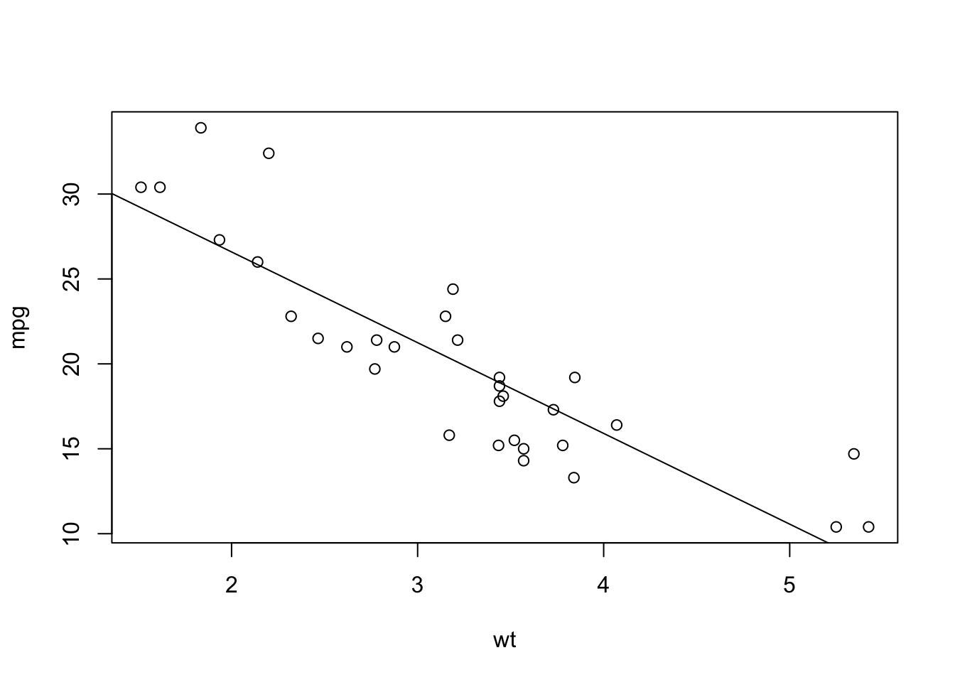

Figure 4.2: A scatterplog between miles per gallon and car weight with regression line.

4.2.3 Specificion issues

I can imagine that you are not very satisfied yet with the analysis. First of all, the relation between mpg and wt might be nonlinear and, secondly, you would like to include additional variables. First we look at the possible nonlinearity in the regression relation (note that we can use the regression formula as before, but that we can specify logarithmic relations by log()):

logmodel <- lm(log(mpg)~log(wt), mtcars)
summary(logmodel)

## 
## Call:
## lm(formula = log(mpg) ~ log(wt), data = mtcars)
## 
## Residuals:
##      Min       1Q   Median       3Q      Max 
## -0.18141 -0.10681 -0.02125  0.08109  0.26930 
## 
## Coefficients:
##             Estimate Std. Error t value Pr(>|t|)    
## (Intercept)  3.90181    0.08790   44.39  < 2e-16 ***
## log(wt)     -0.84182    0.07549  -11.15 3.41e-12 ***
## ---
## Signif. codes:  0 '***' 0.001 '**' 0.01 '*' 0.05 '.' 0.1 ' ' 1
## 
## Residual standard error: 0.1334 on 30 degrees of freedom
## Multiple R-squared:  0.8056, Adjusted R-squared:  0.7992 
## F-statistic: 124.4 on 1 and 30 DF,  p-value: 3.406e-12

We have now the same type of output as before, but I would like to focus on two things here. First, the \(R^2\) has gone up and that is what you typically get in the social sciences. Logarithmically transformed variables usually fit better. Secondly, the interpretation of the estimate now differs. It has become an elasticity with size \(-0.84\), which is quite high again. If the car doubles in weights, the fuel efficiency of the car goes down by 84%!

Secondly, you might want to include other variables, such as being a foreing car (opposite to a car from the US) (vs), the number of cylinders (cyl), the gross horsepower (hp) and how quick the car does over a quarter of a mile (qsec). Again, we are not interested in these additional variables or whether they crank up the \(R^2\). The only thing we are interested is in whether the coefficient of log(wt) changes.

extendedmodel <- lm(log(mpg)~log(wt)+vs+cyl + hp + qsec, mtcars)
summary(extendedmodel)

## 
## Call:
## lm(formula = log(mpg) ~ log(wt) + vs + cyl + hp + qsec, data = mtcars)
## 
## Residuals:
##       Min        1Q    Median        3Q       Max 
## -0.201746 -0.065242 -0.009506  0.079809  0.205166 
## 
## Coefficients:
##               Estimate Std. Error t value Pr(>|t|)    
## (Intercept)  3.5280554  0.4610947   7.651 4.04e-08 ***
## log(wt)     -0.6514583  0.1509786  -4.315 0.000205 ***
## vs          -0.0149215  0.0863277  -0.173 0.864111    
## cyl         -0.0160253  0.0314486  -0.510 0.614651    
## hp          -0.0007670  0.0006861  -1.118 0.273786    
## qsec         0.0212017  0.0267153   0.794 0.434603    
## ---
## Signif. codes:  0 '***' 0.001 '**' 0.01 '*' 0.05 '.' 0.1 ' ' 1
## 
## Residual standard error: 0.1121 on 26 degrees of freedom
## Multiple R-squared:  0.8811, Adjusted R-squared:  0.8582 
## F-statistic: 38.53 on 5 and 26 DF,  p-value: 3.227e-11

Clearly, the coefficient of log(wt) changes with the inclusion of additional variables. So there was unobserved heterogeneity bias in our baseline model (and most likely there still is in our extended model), even though the addional variables are not siginficant.

4.2.4 Reporting

Hopefully you agree that the regression output of above looks horrible and that you do not need all these statistics and stuff. Therefore, you need to construct your own table for presentation format. The minimum what should be in these tables are the coefficient names, the estimates, the standard errors (and the stars would be nice as well), the \(R^2\) and the number of observations used.

Unfortunately, creating tables of your own is a pain in the … Luckily, within R (and by the way in programs as Stata as well) you can do this automatically! In R there are several packages one can use. I prefer the package Stargazer and after using this package we get the following outcome for our logarithmic specification:⁵

stargazer(logmodel, extendedmodel, header=FALSE, type = "html", omit.stat = c("rsq", "f"))


	Dependent variable:

	log(mpg)
	(1)	(2)

log(wt)	-0.842^***	-0.651^***
	(0.075)	(0.151)

vs		-0.015
		(0.086)

cyl		-0.016
		(0.031)

hp		-0.001
		(0.001)

qsec		0.021
		(0.027)

Constant	3.902^***	3.528^***
	(0.088)	(0.461)


Observations	32	32
Adjusted R²	0.799	0.858
Residual Std. Error	0.133 (df = 30)	0.112 (df = 26)

Note:	p<0.1; p<0.05; p<0.01

Note that we now display both specifications, the first the univariate case and the second the multivariate case. This is now typically done in social science research. You start with a baseline and then add variables to check whether the variable of interest remains robust.

4.2.5 Internal validation

So, after done all modeling exercitions you are not done! Now, it is time to validate your results internally. Can you be confident of your results? Or is the parameter that you have found still suspect of possible biases. Here again come the three least squares assumptions:

No large outliers: we have checked that with our descriptive statistics and our scatterplot and it seems that this assumption is met.
Both miles per gallon and car weight should be i.i.d.. We can reasonably assume that the sampling has been done correctly.
The following condition should hold: \(E[\epsilon|X=x] = 0\). This one is dubious. Probably there is no reverse causality (difficult to image that miles per gallon would influence car weight), but most likely there are other factors that impact car weight and miles per gallon which are omitted (where is the car build, what is the car brand, etcetera.). One possible strategy here is to add additional variables until the parameter of interest remains robust (does not change anymore).

Note that the number of observations in this case is only 32, so whether our standard errors are automatically normally distributed is highly questionable, but for the sake of the exposition (and the fact that small sample statistics are very complex) we leave it just with this observation.

To get nice tables directly into Word, you need something else (as you can imagine, because Word is not scriptable). With Stargazer you should give the command as such stargazer(logmodel, extendedmodel, out = "table1.txt",omit.stat = c("rsq", "f")) and thereafter you can read in and edit the table table1.txtin Word.↩